Denition of ICA

\[X = AS\]

• \(X\) is a random \(M \times T\) matrix representing the observed matrix at T time points

• \(S\) is a random \(M \times T\) matrix where each row is mutually independent

• A is an M \(\times\) M full-rank non-random mixing matrix

• Estimate the unmixing matrix \(W = A^{-1}\) such that \(\hat{S}=\hat{W}X\) is the estimates of \(S\).

ICA Assumption 1: Independence

• Definition and fundamental properties: we define that two variables and are independent if and only if the joint pdf is factorizable in the following way: \[p(s_1,s_2 )=p(s_1) p(s_2)\]

• Expected Value Definition (came form moment generating function):
  \[E(h_1(s_1)h_2(s_2))=E(h_1(s_1)) E(h_2(s_2))\] for any functions \(h_1\) and \(h_2\) such that the above expected values exist and are well-defined.

2: Non-Gaussian

• Why Gaussian variables are forbidden? the distribution of any orthogonal transformation of the Gaussian \((s_1,s_2)\) has exactly the same distribution as \((s_1,s_2)\).
• If \(R\) were some arbitrary orthogonal matrix so that \(RR^{\top}=R^{\top}R=I\). Let \(A^{\prime} = AR\). If data had been mixed according to \(A^{\prime}\) (instead of \(A\)), we would have \(X\) as a Gaussian with a mean still 0 and covariance: \[ Cov(X)=E XX^{\top}=E A^{\prime}SS^{\top}{A^{\prime}}^{\top}\]

\[ E ARSS^{\top}R^{\top}A^{\top}=ARR^{\top}A^{\top}=AA^{\top}\]

Measure of Non-gaussianity

• We need to have a quantitative measure of non-gaussianity for ICA Estimation.

• Kurtosis : gauss=0 (sensitive to outliers) \[kurt(Y)=E Y^4 - 3 (EY^2)^2\]

• Entropy : gauss=largest \[H_Y(y)=-\int f_Y(y)\log f_Y(y)dy\]

• Neg-entropy : gauss = 0 \[J(Y)=H(Y_{gaussian})-H(Y)\]

• Approximations \[J(Y) \approx \frac{1}{12}(EY^2)^2 +\frac{1}{48} kurt(Y)^2\]

Caution & Limitation

Example: Data generation

• Two soures were generated from standard normal and Uniform(0,2\(\sqrt{3}\)).

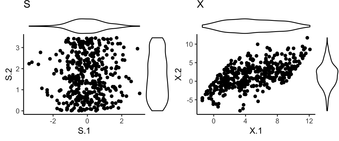
Example: Source separation

• PCA vs. ICA

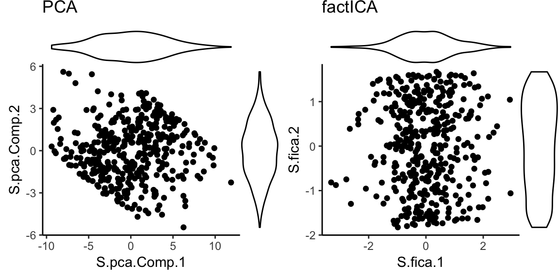
Example: Source separation (Cont.)

• Why PCA could not recover sources while ICA could?

• PCA finds the directions that explains most variance (2nd order), while ICA finds the directions that maximize “independence”.

• If the soures are from normal distribution, finding direction that makes the estimated \(S\) uncorrelated will achieve finding independent sources.

• However, if the sources are not from gaussian distribution, uncorrelation does not mean independence.

• e.g. S1 ~ unif(-1,1)*sqrt(6), S2 ~ exp(1)

• X1=2*S1 + S2; X2=S1-S2: X1 and X2 are uncorrelated, but not independent.

• (X1-X2, X1+2X2) = (S1+2S2, 4S1-S2), Uncorrelated, but not independent.

functional Magnetic Resonance Imaging (fMRI)

• Creates a series of images that capture blood oxygination level dependent (BOLD) signal in parts of the brain

• Non-invasive method

• Popularly used in clinical practice and human brain research

-Find the part of the brain handling certain functions such as movement, sensation, thought, etc.

• Characterize the brain functions

functional Magnetic Resonance Imaging (fMRI) Data

• fMRI volume image. Red and yellow area highlight activated

fMRI Data Matrix

fMRI Data Decomposition

\[X = AS \]

ICA in fMRI

• Relying on the intrinsic structure of the data

• No assumptions about the form of the HRF or the possible causes of responses are made.

• The only assumption is mutual independence in “Space” (spatial ICA) or in “Time” (temporal ICA).

Temporal vs. Spatial ICA}

Temporal vs. Spatial ICA

Real example data

• Dataset was downloaded from FSL (https://fsl.fmrib.ox.ac.uk/fslcourse/)

• Demostrate run ICA in fsl and R, and how to look at the results.

• Dataset was “preprocessed” using FSL FEAT (default setting)

library(fslr)
img = readnii('ica_intro_fsldata/filtered_func_data.nii.gz'); 
print(img)

## NIfTI-1 format
##   Type            : nifti
##   Data Type       : 4 (INT16)
##   Bits per Pixel  : 16
##   Slice Code      : 0 (Unknown)
##   Intent Code     : 0 (None)
##   Qform Code      : 1 (Scanner_Anat)
##   Sform Code      : 1 (Scanner_Anat)
##   Dimension       : 64 x 64 x 21 x 100
##   Pixel Dimension : 4 x 4 x 6 x 1
##   Voxel Units     : mm
##   Time Units      : sec

One volume

Five random voxels

ts.plot(t(img[c(25,30,35,40,45),32,10,]),col=1:5)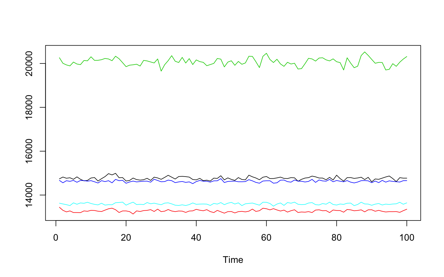

Five random voxels

ts.plot(scale(t(img[c(25,30,35,40,45),32,10,])),col=1:5)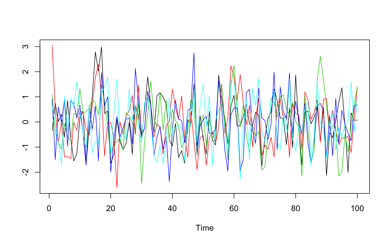

How to apply ICA

• The easiest way is to use a neuroimage package such as FSL-Melodic, GIFT, etc.

• In R, f.ica.fmri function is available in AnalyzeFMRI R package.

• Typically spatial ICA is applied for FMRI, and temporal ICA is applied to EEG.

• The basic steps include: array flattening, prewhitening, optimization (estiomation), spatial/temporal component recovery

Practice (Spatial ICA):

• Flattening 4D volumes to 2D (V \(\times\) T) matrix

dims=dim(img)
X=t(array(img, dim=c(dims[1]*dims[2]*dims[3],dims[4])))
X.c = X - apply(X,1,mean)

• Prewhitening

• Select number of components (in fMRI application it is often set to be 20, but there’s also some systematic way to determine).

Sigma.eigen=svd(X.c)
n.comp=10
Y = t(Sigma.eigen$v[,1:n.comp]) 

spatial ICA example (Cont.)

• ICA is applied to Y

set.seed(1234)
system.time(re<-fastICA(t(Y),10))

##    user  system elapsed 
##   2.592   0.871   3.472

temporal component recoveray

A.est = Sigma.eigen$u[,1:n.comp] %*% re$A
ts.plot(scale(A.est),col=1:10)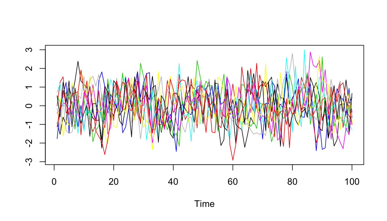

IC1

par(mfrow=c(1,2))
ts.plot(scale(A.est[,1]),col=1:10,ylab='')
map1=array(scale(re$S[,1]),dim=dims[1:3])
image(map1[,,10],breaks=c(-100:100)/100*21,col=bluered(200),xaxt='n',yaxt='n')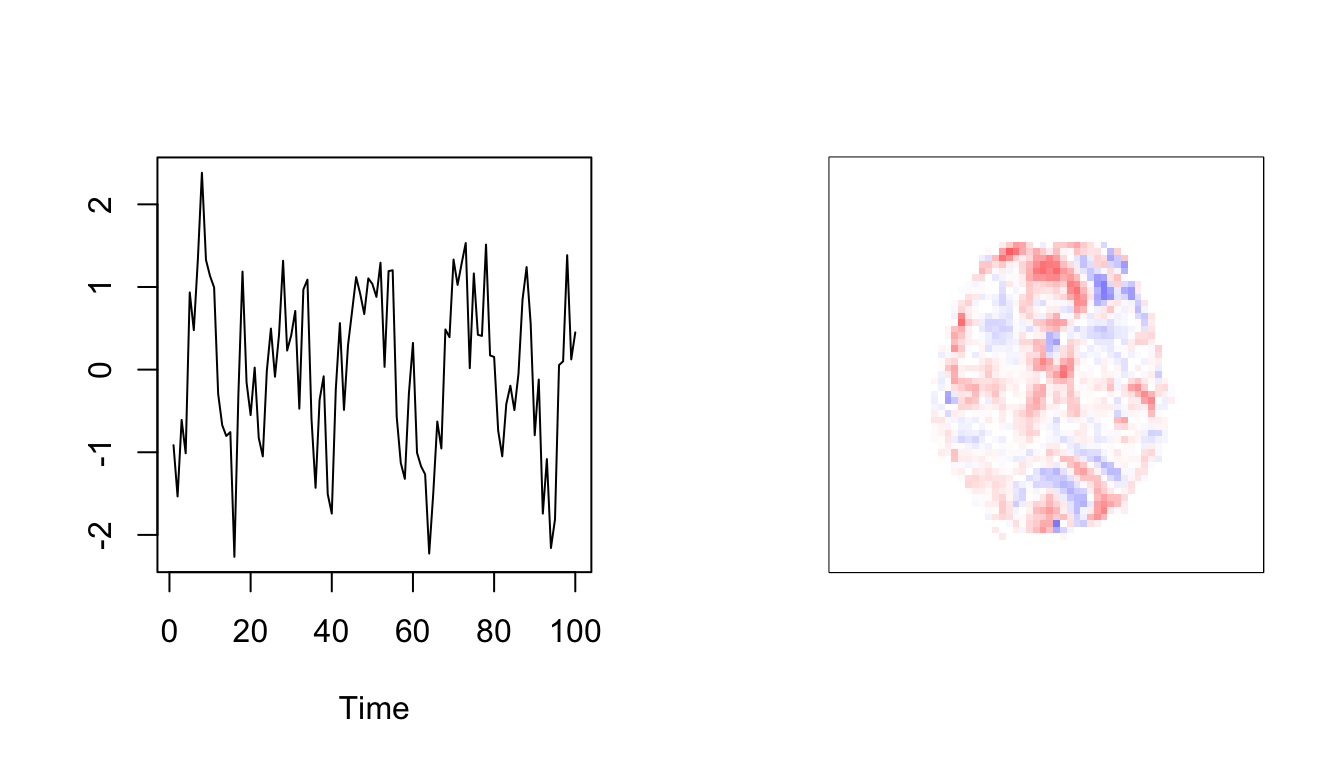

IC5,10

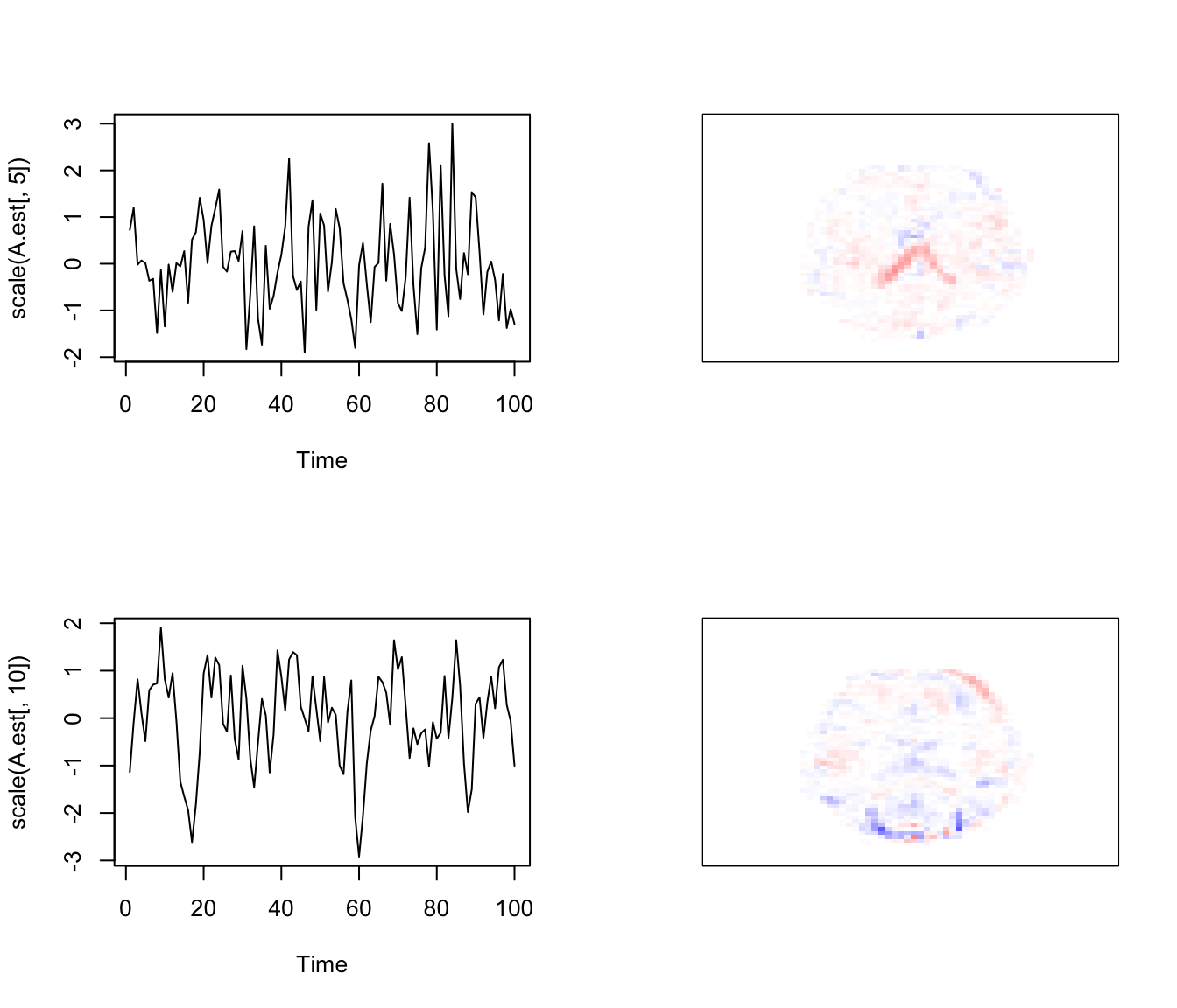
Some note.

• fastICA has built in prewhitening!

• Unfortunately, it won’t give you exactly same answer because the algorithm is stochastic! (due to optimization)

• A lot of ICA algorithms are designed to have random initialization (like K-means clustering). They often gives similar answers, but not always. Have to be cautious.

library(fastICA)

set.seed(1235)
system.time(re2<-fastICA(t(X.c),n.comp=10))
image(cor(cbind(re$S, re2$S))[1:10,1:10+10],
      col=bluered(200),breaks=c(-100:100)/100)

Conclusion

• We will discuss group ICA and advanced ICAs (longitudinal ICA) next week!