Dynamic Functional Connectom

Motivation

2019 summer plan research them~/

Functional Connectivity – Literature review for functional connectivity – Analyze RANN/CR/ADNI non-task and task fMRI data
Interpretable machine learning – Literature review and analysis for anxiety project
Independent component analysis – Group level analysis for EEG and resting state data

Today:

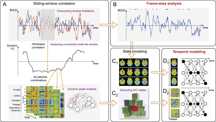
Soft introduction of (dynamic) functional connectivity (dFC) (Preti, Bolton, and Van De Ville 2017)
Some example of the most popularly used dFC method

Functional connectivity

Functional connectivity (FC):

the temporal correlation (often measured as a Pearson’s r) in the high amplitude, low-frequency spontaneously generated BOLD signal between voxels (cubic “pixel” in a three-dimensional brain image) or brain regions (Fox & Raichle, 2007)

Why dynamic connectivity?

FC has been shown to fluctuate over time.

Many of existing dFC Mmethods are too complicated:

Due to the inherent sophistication of methods designed to track temporal fluctuations, it is sometimes difficult to clearly evaluate the underlying hypotheses and validity of a dFC technique in a given setting.

Suggested future directions (by the authors):

focusing on a subset of temporally sparse activation events in place of windowed connectivity estimates, and understanding how time should be modeled in the description of connectivity changes.

2. Dynamic functional connectivity: Sliding window approach

fMRI data are preprocessed using preprocessing pipeline (e.g. fsl, spm, afni, etc,) including coregistration, low/high pass filtering, motion correction, slice time correction.

Sliding window approach

Correlation matrix over the sliding windows.

Pearson correlation between pairs of the timecourses is computed over a temporal interval spanned by a rectangular window. This computation is repeated iteratively, shifting the window by a specific step every time, to generate a connectivity timecourse.

Real Data Example

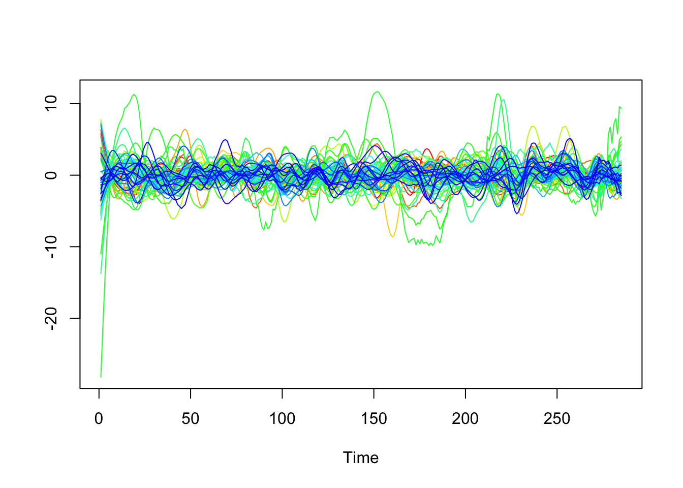
Using Gorden template, mean time series from 333 ROIs from 26 functional networks are extracted.
One subject from RANN/CR study, non-task fMRI

FC

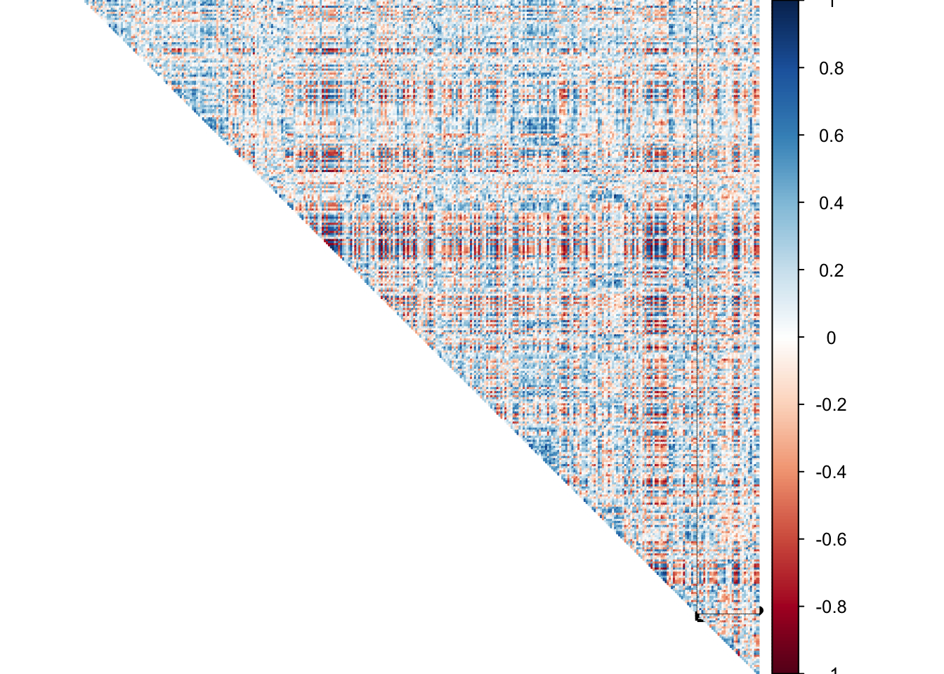
Pearson’s correlation is computed between 333 time series.

Sliding window

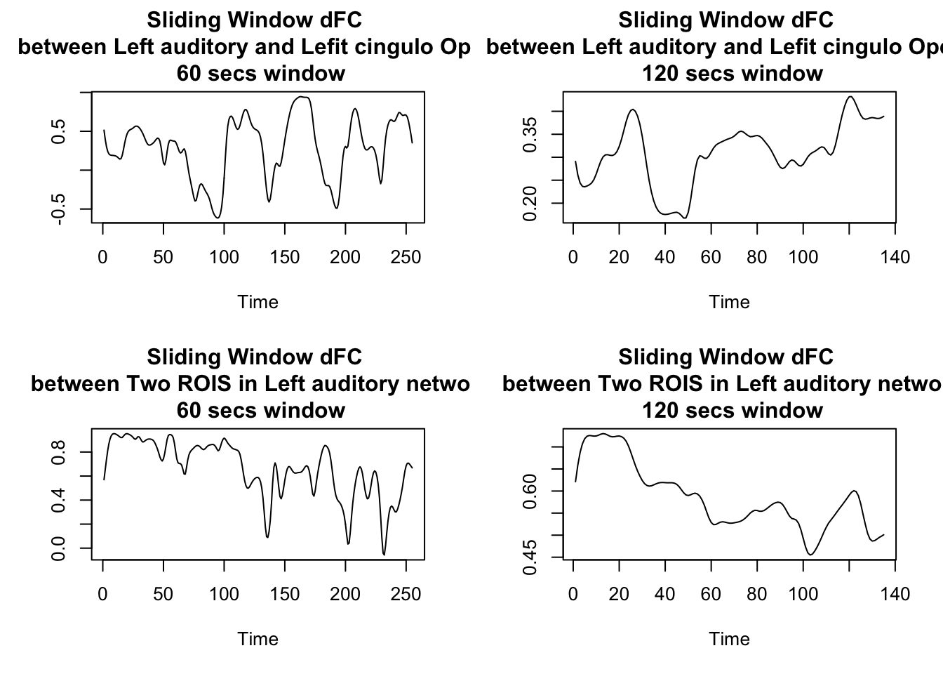
Set the window as 60 secs (equivalent to 30 time points) vs. 120 secs (60 time points)

Limitations

Too small window: potentially include artifacts
Too large window: cannot detect temporal dynamics
Time-frequency approach: allows exploring connectivities in different frequencies, but too much information
Rule of thumb: 30-60s, but the big issue is we ended up computing correlation only using few time points.
Rectangular window: gives same weights within the window; sensitive to outliers
Solution 1: tapered windows: gives different weights (e.g. less weights to the border), still depends on the preselection of the window size
Solution 2: data-driven window selection (e.g. regression-based change point detection; finding windows preserve local stationariy).
still very ambiguous about how we model this dFC to associated with outcomes of interest, potentially how we can jointly model spatial and temporal patterns of dFC simultaneously. That will be the topic we will expore this summer.

References

Preti, Maria Giulia, Thomas AW Bolton, and Dimitri Van De Ville. 2017. “The Dynamic Functional Connectome: State-of-the-Art and Perspectives.” Neuroimage 160:41–54.